################################################################################
# Script Name: process.r
# Description: Analyse descriptive des mobilités résidentielles en finistère
# entre 2020 et l'années de résidence prédédent. Données de l'INSEE.
# Ce script est dédié à la cartograpie des indices calculés dans le
# script `scripts/process.r`
# Author: Antoine Le Doeuff
################################################################################
library(readr)
library(sf)
library(dplyr)
library(Matrix)
library(ggplot2)
library(ggspatial)
library(ggnewscale)
library(patchwork)
library(ttt) # remotes::install_github("MiboraMinima/ttt")
library(mapsf)
library(ggtext)
# //////////////////////////////////////////////////////////////////////////////
# Constantes -------------------------------------------------------------------
# Où sont enregistré les données (vous, ce sera juste `data`)
DATA_DIR <- "02_flux/data"
# Où seront enregistrées vos cartes (vous, ce sera juste `figures`)
FIGURES_DIR <- "02_flux/figures"
# //////////////////////////////////////////////////////////////////////////////
# Chargement des données -------------------------------------------------------
# Le tableau des mobilités résidentielles filtées
dt_mobi_fin <- read_csv(glue::glue("{DATA_DIR}/res/mobi_res_29.csv"))
# Table des indices spatiaux
indices_spa <- read_sf(glue::glue("{DATA_DIR}/res/indices_spa_29.gpkg"))
# Communes du finistères
coms <- read_sf(glue::glue("{DATA_DIR}/src/com_finistere_bdtopov3_2026.gpkg"))
# Matrice des relations préférentielles
m_pref <- readRDS(glue::glue("{DATA_DIR}/res/rel_pref.rds"))
# //////////////////////////////////////////////////////////////////////////////
# Prétraitements ---------------------------------------------------------------
# Calcul des centroïdes (pour les cartes en cercles proportionnelles)
centroids <- st_centroid(indices_spa)
# //////////////////////////////////////////////////////////////////////////////
# Cartographie -----------------------------------------------------------------
# Themes .......................................................................
# Je crée un thème que j'appliquerai à toutes les cartes
sysfonts::font_add_google(name = "Roboto", family = "roboto")
theme_ggplot <-
theme_minimal() +
theme(
legend.position = "bottom",
# La font chargé dans `text` est automatiquement appliquée à tous les
# autres texts de l'objet ggplot. Vous pouvez la changer manuellement
# pour un paramètre en particulier si vous le shouaitez.
text = element_text(family = "roboto"),
plot.title = ggtext::element_markdown(size = 16, face = "bold"),
plot.subtitle = ggtext::element_markdown(size = 12, lineheight = 1.2),
axis.title.x = ggtext::element_markdown(size = 12),
axis.title.y = ggtext::element_markdown(size = 12),
plot.caption = ggtext::element_markdown(size = 8, lineheight = 1.5),
legend.title = ggtext::element_markdown(size = 8)
)
# Theme pour patchwork
theme_patch <-
theme(
text = element_text(family = "roboto"),
plot.title = element_text(face = "bold", size = 18),
plot.subtitle = ggtext::element_markdown(size = 14, lineheight = 1.2),
plot.caption = ggtext::element_markdown(size = 11)
)
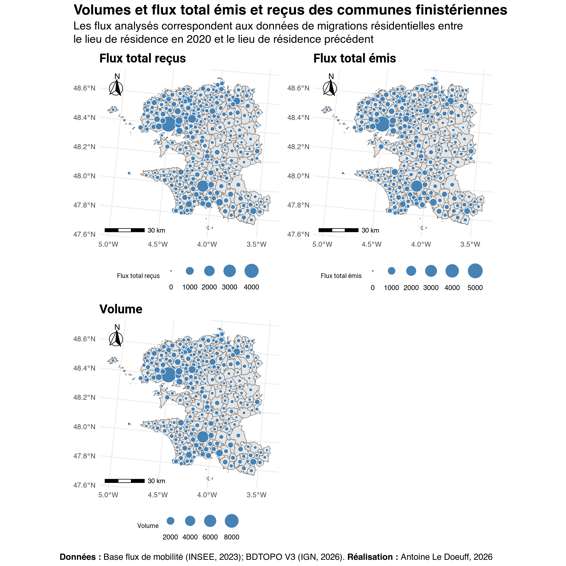
# Plot departure, arrival, volumes .............................................
# On défini le nom complet de le la variable avec un named vector
selected_vars <- c(
"Flux total reçus" = "arrival",
"Flux total émis" = "departure",
"Volume" = "volumes"
)
# On définit une liste vide (réceptacle qui va recevoir les cartes)
maps <- list()
# On itère sur les noms
for (name in names(selected_vars)) {
# On récupère le nom présent dans le tableau à partir du nom complet
short_name <- selected_vars[name]
# Créée la carte
m <- ggplot() +
geom_sf(data = coms) +
geom_sf(
data = centroids,
aes(size = .data[[short_name]]),
pch = 21, fill = "steelblue", color = "white"
) +
scale_size(
name = name,
range = c(1, 9),
breaks = scales::pretty_breaks(n = 5)
) +
ggtitle(name) +
ggspatial::annotation_scale(
location = "bl", height = unit(0.15, "cm")
) +
ggspatial::annotation_north_arrow(
location = "tl", which_north = "true",
height = unit(1, "cm"), width = unit(1, "cm"),
style = north_arrow_fancy_orienteering
) +
guides(
size = guide_legend(
direction = "horizontal",
nrow = 1,
label.position = "bottom"
)
) +
theme_ggplot
maps[[name]] <- m
}
# Je combine les graphs et je fais la mise en page de la carte finale
map_volumes_emis_recus <- patchwork::wrap_plots(maps, ncol = 2) +
plot_annotation(
title = "Volumes et flux total émis et reçus des communes finistériennes",
subtitle = "Les flux analysés correspondent aux données de migrations résidentielles entre<br>le lieu de résidence en 2020 et le lieu de résidence précédent",
caption = "**Données :** Base flux de mobilité (INSEE, 2023); BDTOPO V3 (IGN, 2026). BDTOPO V3 (IGN, 2026). **Réalisation :** Antoine Le Doeuff, 2026",
theme = theme_patch
)
# J'enregistre la carte
ggsave(
glue::glue("{FIGURES_DIR}/map_volumes_emis_recus.png"),
map_volumes_emis_recus,
width = 21 - 1, # Largeur en cm (A4 moins 1 cm pour la marge)
height = 27 - 1,
units = "cm", dpi = 300
)
# J'enregistre la carte en .eps ou svg ou pdf (pour pouvoir la modifier avec
# logiciel de DAO a prosteriori)
ggsave(
glue::glue("{FIGURES_DIR}/map_volumes_emis_recus.eps"),
map_volumes_emis_recus,
width = 21 - 1, # Largeur en cm (A4 moins 1 cm pour la marge)
height = 27 - 1,
units = "cm"
)
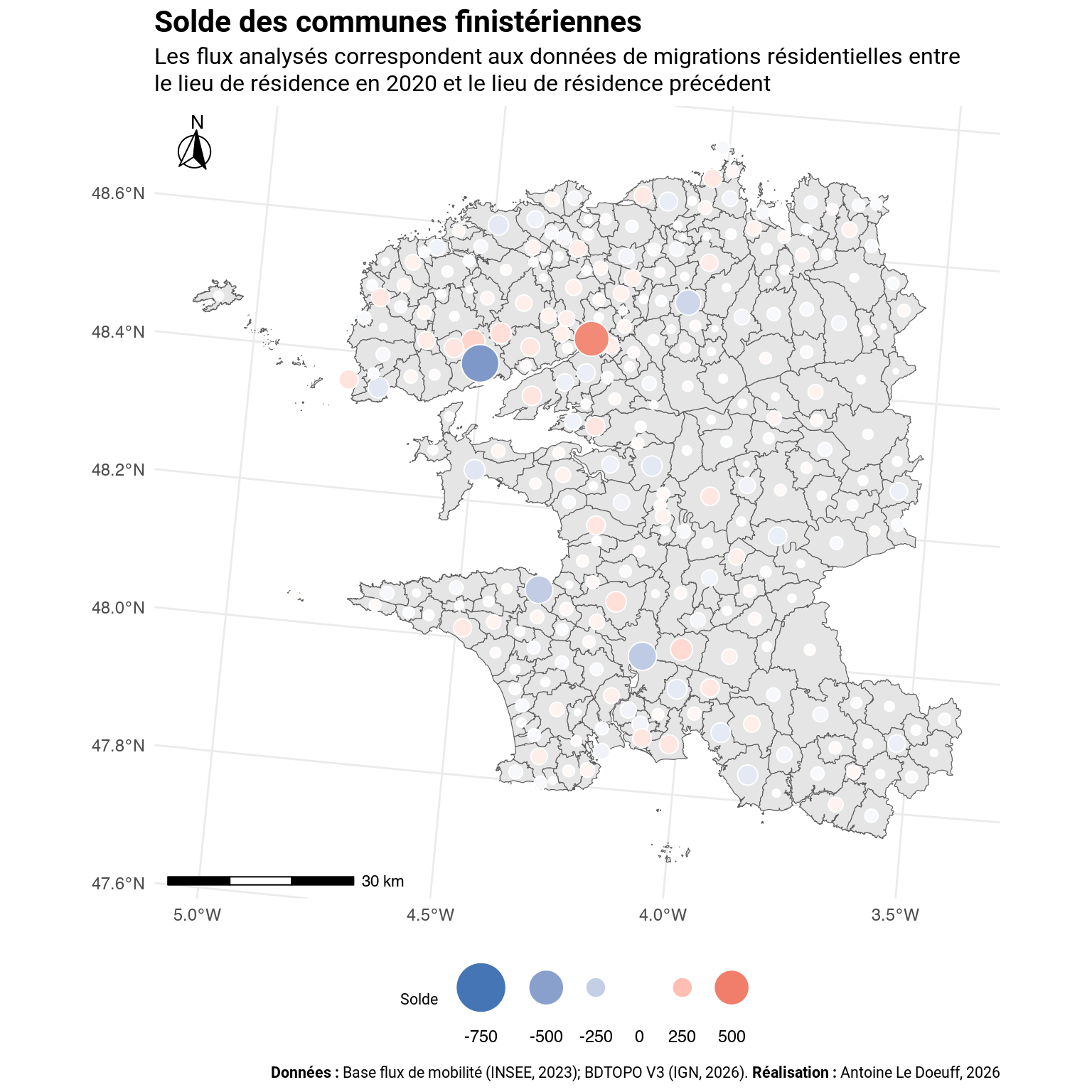
# Solde ........................................................................
# Création de la taille des cercles à la main
fill_breaks <- c(-750, -500, -250, 0, 250, 500)
max_val <- max(abs(centroids$soldes), na.rm = TRUE)
legend_sizes <- scales::rescale(abs(fill_breaks), to = c(1, 9), from = c(0, max_val))
map_solde <- ggplot() +
geom_sf(data = coms) +
geom_sf(
data = centroids,
aes(size = abs(soldes), fill = soldes),
pch = 21, color = "white"
) +
# Cacher la taille dans la légende
scale_size(range = c(1, 9), guide = "none") +
scale_fill_gradient2(
name = "Solde",
low = "#4575B4",
mid = "white",
high = "#D73027",
midpoint = 0,
space = "Lab",
breaks = fill_breaks,
limits = c(-750, 500),
guide = "legend"
) +
guides(
fill = guide_legend(
direction = "horizontal",
nrow = 1,
label.position = "bottom",
# Mettre la taille directement ici
override.aes = list(size = legend_sizes)
)
) +
labs(
title = "Solde des communes finistériennes",
subtitle = "Les flux analysés correspondent aux données de migrations résidentielles entre<br>le lieu de résidence en 2020 et le lieu de résidence précédent",
caption = "**Données :** Base flux de mobilité (INSEE, 2023); BDTOPO V3 (IGN, 2026). BDTOPO V3 (IGN, 2026). **Réalisation :** Antoine Le Doeuff, 2026"
) +
ggspatial::annotation_scale(
location = "bl", height = unit(0.15, "cm")
) +
ggspatial::annotation_north_arrow(
location = "tl", which_north = "true",
height = unit(1, "cm"), width = unit(1, "cm"),
style = north_arrow_fancy_orienteering
) +
theme_ggplot
ggsave(
glue::glue("{FIGURES_DIR}/map_solde.png"),
map_solde,
width = 20 - 1,
height = 20 - 1,
units = "cm", dpi = 300
)
ggsave(
glue::glue("{FIGURES_DIR}/map_solde.pdf"),
map_solde,
width = 20 - 1,
height = 20 - 1,
units = "cm"
)
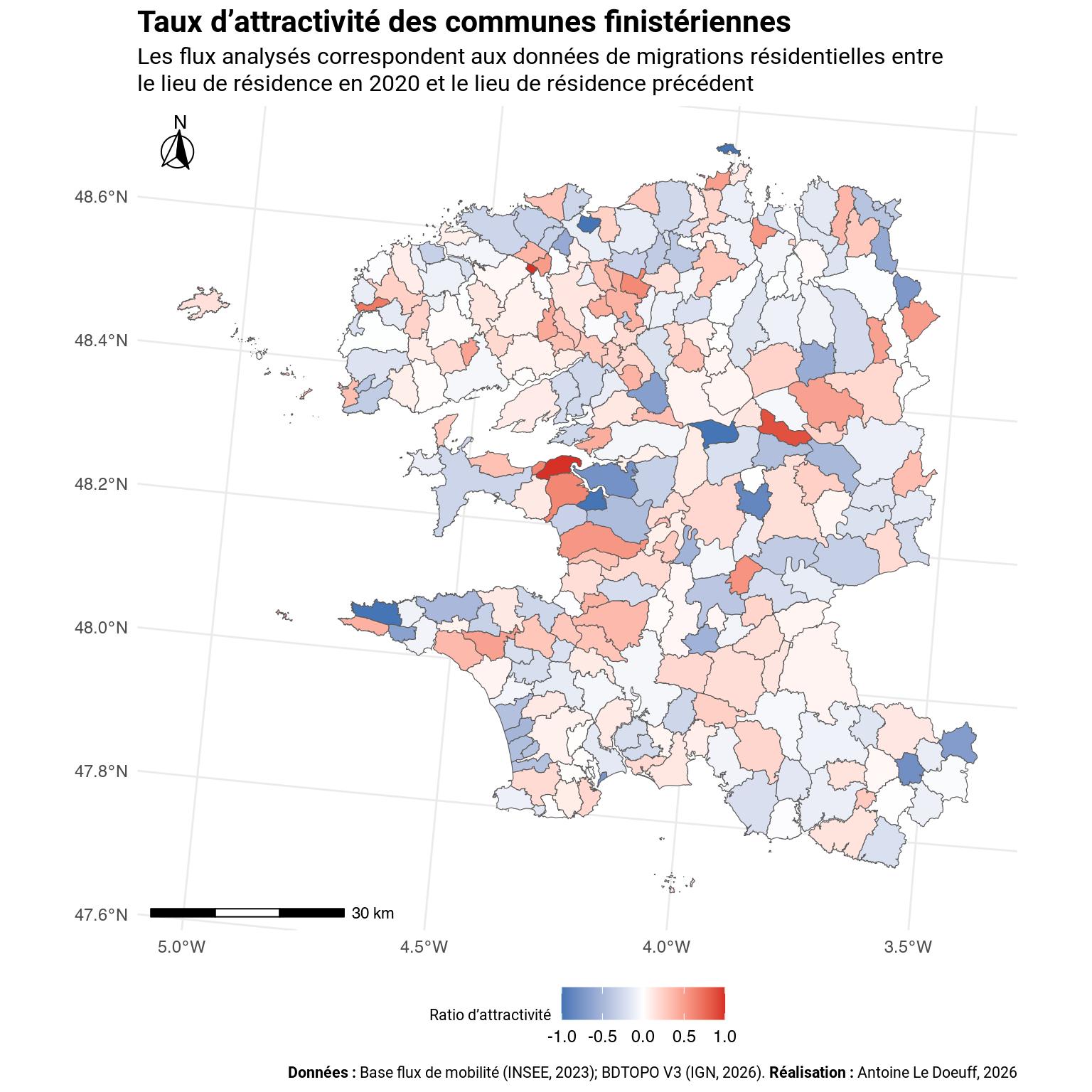
# Attractivity .................................................................
map_attrac_ratio <- ggplot() +
geom_sf(
data = indices_spa,
aes(fill = attrac_ratio), # use transformed color
pch = 21
) +
scale_fill_gradient2(
name = "Ratio d'attractivité",
low = "#4575B4", # blue for negatives
mid = "white",
high = "#D73027", # red for positives
midpoint = 0, # ensures 0 stays white
space = "Lab"
) +
labs(
title = "Taux d'attractivité des communes finistériennes",
subtitle = "Les flux analysés correspondent aux données de migrations résidentielles entre<br>le lieu de résidence en 2020 et le lieu de résidence précédent",
caption = "**Données :** Base flux de mobilité (INSEE, 2023); BDTOPO V3 (IGN, 2026). BDTOPO V3 (IGN, 2026). **Réalisation :** Antoine Le Doeuff, 2026"
) +
ggspatial::annotation_scale(
location = "bl", height = unit(0.15, "cm")
) +
ggspatial::annotation_north_arrow(
location = "tl", which_north = "true",
height = unit(1, "cm"), width = unit(1, "cm"),
style = north_arrow_fancy_orienteering
) +
theme_ggplot
ggsave(
glue::glue("{FIGURES_DIR}/map_attrac_ratio.png"),
map_attrac_ratio,
width = 20 - 1,
height = 20 - 1,
units = "cm", dpi = 300
)
ggsave(
glue::glue("{FIGURES_DIR}/map_attrac_ratio.eps"),
map_attrac_ratio,
width = 20 - 1,
height = 20 - 1,
units = "cm"
)
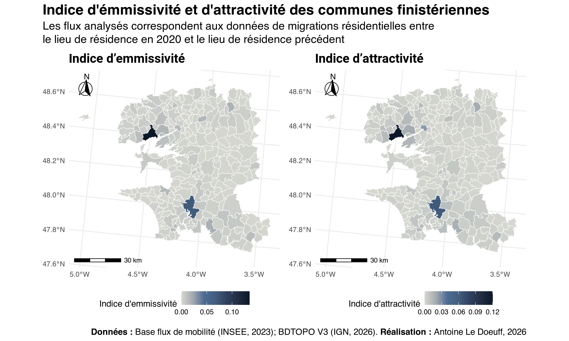
# Indices d'emmissivité et d'attractivité ......................................
to_plot_vars <- c("Indice d'emmissivité" = "ie", "Indice d'attractivité" = "ia")
maps <- list()
for (name in names(to_plot_vars)) {
short_name <- to_plot_vars[name]
m <- ggplot() +
geom_sf(
data = indices_spa,
aes(fill = .data[[short_name]]),
color = "white",
pch = 21
) +
scale_fill_gradientn(
name = name,
colors = MexBrewer::mex.brewer("Frida"),
) +
labs(title = name) +
ggspatial::annotation_scale(
location = "bl", height = unit(0.15, "cm")
) +
ggspatial::annotation_north_arrow(
location = "tl", which_north = "true",
height = unit(1, "cm"), width = unit(1, "cm"),
style = north_arrow_fancy_orienteering
) +
theme_minimal() +
theme(
legend.position = "bottom",
plot.title = ggtext::element_markdown(family = "roboto", size = 16, face = "bold"),
plot.subtitle = ggtext::element_markdown(family = "roboto", size = 12, lineheight = 1.2),
axis.title.x = ggtext::element_markdown(family = "roboto", size = 12),
axis.title.y = ggtext::element_markdown(family = "roboto", size = 12),
plot.caption = ggtext::element_markdown(family = "roboto", size = 8, lineheight = 1.5)
)
maps[[short_name]] <- m
}
map_ia_ie <- patchwork::wrap_plots(maps) +
plot_annotation(
title = "Indice d'émmissivité et d'attractivité des communes finistériennes",
subtitle = "Les flux analysés correspondent aux données de migrations résidentielles entre<br>le lieu de résidence en 2020 et le lieu de résidence précédent",
caption = "**Données :** Base flux de mobilité (INSEE, 2023); BDTOPO V3 (IGN, 2026). BDTOPO V3 (IGN, 2026). **Réalisation :** Antoine Le Doeuff, 2026",
theme = theme_patch
)
ggsave(
glue::glue("{FIGURES_DIR}/map_ia_ie.png"),
map_ia_ie,
width = 21 - 1, # Largeur en cm (A4 moins 1 cm pour la marge)
height = 27 - 1,
units = "cm", dpi = 300
)
ggsave(
glue::glue("{FIGURES_DIR}/map_ia_ie.eps"),
map_ia_ie,
width = 21 - 1, # Largeur en cm (A4 moins 1 cm pour la marge)
height = 27 - 1,
units = "cm"
)
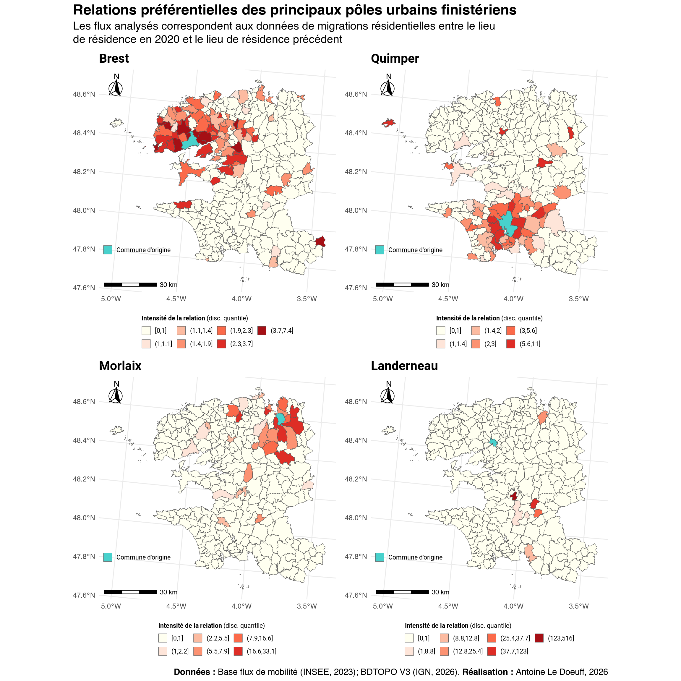
# Relations préférentielles ....................................................
# Conversion de la matrice des relations préférentielles en data.frame
od_tidy <- as.data.frame(as.matrix(m_pref)) |>
tibble::rownames_to_column("origin") |>
tidyr::pivot_longer(
cols = -origin,
names_to = "destination",
values_to = "rel_pref"
)
# Les communes que je souhaites cartographier
coms_to_plot <- c(
"Brest" = "29019",
"Quimper" = "29232",
"Morlaix" = "29151",
"Landerneau" = "29041"
)
# Seuil de définition d'un relation préférentielle. Les relations inférieure à
# ce seuil ne seront pas cartographiées.
th <- 1
# Filtre du df des rel. pref. pour ne garder que les communes sélectionnées
# Ne garder que les communes sélectionnées
to_plot <- filter(od_tidy, origin %in% coms_to_plot)
# On récupère les géométries
to_plot <- left_join(indices_spa, to_plot, by = c("code_insee" = "destination"))
maps <- list()
for (com_name in names(coms_to_plot)) {
ci <- coms_to_plot[com_name]
data_current_com <-
filter(to_plot, origin == ci) |>
select(origin, rel_pref)
# discrétisation quantile
breaks <- quantile(
pull(filter(data_current_com, rel_pref > th), rel_pref),
probs = seq(0, 1, by = 0.2),
na.rm = TRUE
)
# Ajouter la légende pour les valeurs < th (on round pour la légende)
breaks <- round(c(0, 1, breaks), 1)
# Créer une variable avec le seuil des quantiles
data_current_com <- data_current_com |>
mutate(
rel_pref_q = cut(
round(rel_pref, 1), # Il faut round ici aussi
breaks = unique(breaks),
include.lowest = TRUE,
dig.lab = 3
)
)
m <- ggplot() +
geom_sf(data = data_current_com, aes(fill = rel_pref_q)) +
scale_fill_manual(
name = "**Intensité de la relation** (disc. quantile)",
# Mettre une couleur partiuclière pour les valeurs < 1 (th)
values = c("ivory", RColorBrewer::brewer.pal(6, "Reds")),
na.value = "grey90",
guide = guide_legend(
position = "bottom",
direction = "horizontal",
title.position = "top",
nrow = 2
)
) +
new_scale_fill() +
geom_sf(
data = filter(coms, nom_officiel == com_name),
aes(fill = "Commune d'origine")
) +
scale_fill_manual(
name = NULL,
values = c("Commune d'origine" = "mediumturquoise"),
guide = guide_legend(position = "inside")
) +
labs(title = com_name) +
ggspatial::annotation_scale(location = "bl", height = unit(0.15, "cm")) +
ggspatial::annotation_north_arrow(
location = "tl", which_north = "true",
height = unit(1, "cm"), width = unit(1, "cm"),
style = north_arrow_fancy_orienteering
) +
theme_ggplot +
theme(
legend.position.inside = c(0, 0.15),
legend.justification.inside = c(0, 0),
legend.key.size = unit(0.4, "cm"),
legend.text = element_text(family = "roboto", size = 8),
legend.background = element_rect(fill = NA, color = NA)
)
maps[[com_name]] <- m
}
map_rel_pref <- patchwork::wrap_plots(maps, ncol = 2) +
plot_annotation(
title = "Relations préférentielles des principaux pôles urbains finistériens",
subtitle = "Les flux analysés correspondent aux données de migrations résidentielles entre le lieu<br>de résidence en 2020 et le lieu de résidence précédent",
caption = "**Données :** Base flux de mobilité (INSEE, 2023); BDTOPO V3 (IGN, 2026). BDTOPO V3 (IGN, 2026). **Réalisation :** Antoine Le Doeuff, 2026",
theme = theme_patch
)
ggsave(
glue::glue("{FIGURES_DIR}/map_rel_pref.png"),
map_rel_pref,
width = 21 - 1,
height = 27 - 1,
units = "cm", dpi = 300
)
ggsave(
glue::glue("{FIGURES_DIR}/map_rel_pref.eps"),
map_rel_pref,
width = 21 - 1,
height = 27 - 1,
units = "cm"
)
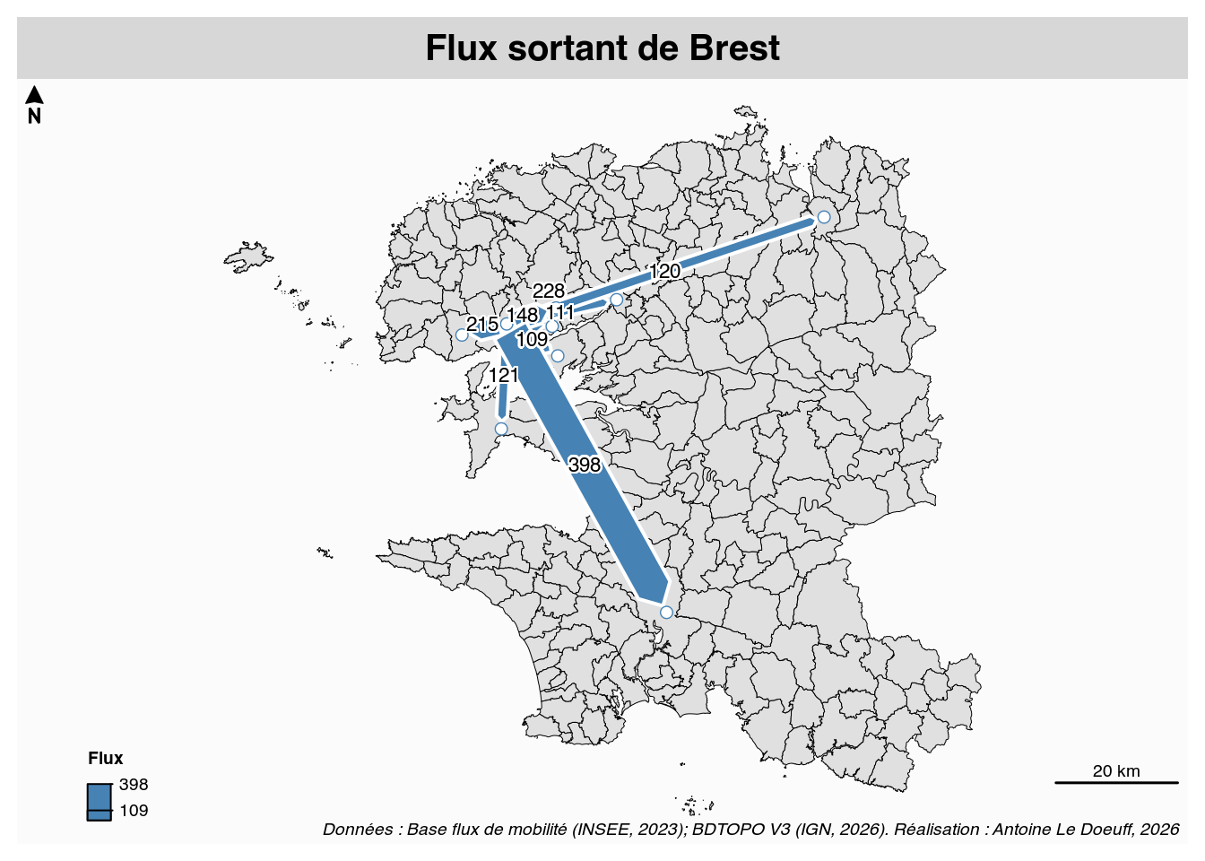
# Flux map .....................................................................
# [Prétraitements]
indices_spa$code_insee <- as.numeric(indices_spa$code_insee)
indices_spa$id <- indices_spa$code_insee
dtp <-
select(dt_mobi_fin, -i, -j) |>
mutate(i = as.numeric(codgeo), j = as.numeric(dcran), fij = nbflux_c20_pop01p) |>
select(i, j, fij)
# [Paramètres]
# Les flux associées à la commune
com_name <- "Brest"
# Le type de flux que l'on souhaite cartographier
type <- "sortant" # "entrant"
# Récupération du code INSEE associé à la commune
ci <- unique(pull(filter(coms, nom_officiel == com_name), code_insee))
# Seuil pour cartographier les flux
th <- 100
# Couleur des lignes
col <- "steelblue"
# Couleur du fond de carte
col_back <- "#E0E0E0"
# [Carto]
# Récupérer tous les flux entrants ou sortants associés à la commune
# et filrer les flux < au seuil.
if (type == "entrant") {
dt_plot <- filter(dtp, j == as.numeric(ci), fij > th)
} else {
dt_plot <- filter(dtp, i == as.numeric(ci), fij > th)
}
# Créer un df avec les communes qui échange des flux
indices_spa_f <-
filter(indices_spa, id %in% unique(c(dt_plot$i, dt_plot$j))) |>
select(id)
# On enregistre ici l'endroit où va être sauvegardé la carte
mf_png(
x = coms,
filename = glue::glue("{FIGURES_DIR}/map_oursin_{type}_{com_name}.png"),
width = 20 - 1, height = 20 - 1, unit="cm"
)
mf_map(
coms,
col = col_back,
border = "black",
lwd = 0.5
)
flows <- ttt_flowmapper(
x = indices_spa_f,
df = dt_plot,
dfid = c("i", "j"),
dfvar = "fij",
xid = "id",
size = "thickness",
type = "arrows",
decreasing = FALSE,
# Configuration des lignes
col = col, # couleur des arcs
border = "white", # couleur du contour
lwd = 2, # épaisseur du contour
k = 15, # augmenter ou diminuer l'épaisseur des arcs
# Configuration des cercles
col2 = "white", # couleur du cercle
border2 = col, # couleur du contour
lwd2 = 0.7, # épaisseur du contour
k2 = 1e3L, # augmenter ou diminuer la taille des cercles
add = TRUE
)
# Ajouter la valeur du flux sur les arcs
# Si vous voulez les enlevez, commentez le code.
flows_txt <- mutate(flows$flows, fij = round(fij, 0)) |> distinct()
mf_label(
flows_txt,
var = "fij",
halo = TRUE,
cex = 0.7,
col = "black",
bg = "white",
r = 0.1,
overlap = FALSE,
lines = FALSE
)
# La légende
ttt_flowmapperlegend(
x = flows,
title = "Flux",
col = col,
txtcol = 'black',
title.cex = 0.6, # Taille du titre de la légende
hshift = 3e3 # Espace entre le titre et légende
)
mf_title(
txt = glue::glue("Flux {type} de {com_name}"),
bg = "#d7d7d7", fg = "black", pos = "center"
)
mf_credits(
txt = "Données : Base flux de mobilité (INSEE, 2023); BDTOPO V3 (IGN, 2026). BDTOPO V3 (IGN, 2026). Réalisation : Antoine Le Doeuff, 2026",
col = "black", pos = "bottomright"
)
mf_arrow(col="black")
mf_scale(col="black", pos="bottomright", adj = c(0, 10))
dev.off() # Indique l'enregistrement de la carte avec les paramètres indiqués dans mf_png()