################################################################################
# Script Name: centro_usa.r
# Description: Analyse centrographique de la population des USA entre 1790 et 2024
# Author: Antoine Le Doeuff
# Date created: 2025-10-28
################################################################################
library(readr)
library(sf)
library(dplyr)
library(rnaturalearth)
library(gganimate)
library(ggplot2)
library(patchwork)
# //////////////////////////////////////////////////////////////////////////////
# Chargement des données -------------------------------------------------------
# Données de pop
# https://www.kaggle.com/datasets/rolfhendriks/us-population-by-state-comprehensive-data
dt <- read_csv("01_points/data/src/us_population_by_state.csv")
# Polygones des USA
# Convertion en NAD83 / Conus Albers Equal Area Projection
states <- ne_states(country = "United States of America", returnclass = "sf") |>
st_transform(crs = 5070)
# //////////////////////////////////////////////////////////////////////////////
# Prétraitements ----------------------------------------------------------------
# Suppression de certains états ................................................
to_remove <- c("Hawaii", "Alaska")
dt <- filter(dt, !state %in% to_remove)
states <- filter(states, !name %in% to_remove)
# Calcul des centroïdes ........................................................
state_centroids <-
st_centroid(states) |>
mutate(
x = st_coordinates(geometry)[,1],
y = st_coordinates(geometry)[,2]
) |>
st_drop_geometry() |>
select(name, x, y)
# Jointure .....................................................................
data_joined <- left_join(dt, state_centroids, by = c("state" = "name"))
# //////////////////////////////////////////////////////////////////////////////
# Analyse centrographique ------------------------------------------------------
# Centre non-pondéré ...........................................................
center_unpondered <- state_centroids |>
summarise(
c_x = mean(x),
c_y = mean(y),
c_sd = sqrt(var(x) + var(y)),
)
# Centre pondéré pour chaque année .............................................
center_pondered <- data_joined |>
  group_by(year) |>
  summarise(
    cw_x = sum(population * x) / sum(population),
    cw_y = sum(population * y) / sum(population),
    cw_sd = sqrt(sum(population * ((x - mean(cw_x))^2 + (y - mean(cw_y))^2)) / sum(population))
  )
# //////////////////////////////////////////////////////////////////////////////
# Analyse ----------------------------------------------------------------------
# Centre pondéré ...............................................................
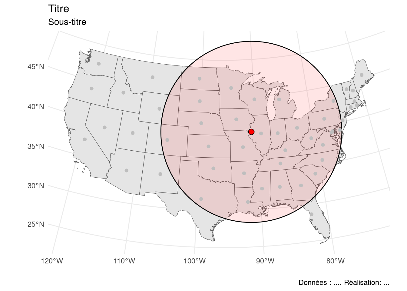
map_unpondered <- ggplot() +
geom_sf(data = states) +
ggforce::geom_circle(
data = center_unpondered,
aes(x0 = c_x, y0 = c_y, r = c_sd),
fill = "red", alpha = 0.1, inherit.aes = FALSE
) +
geom_point(
data = state_centroids,
aes( x = x, y = y),
color = "grey"
) +
geom_point(
data = center_unpondered,
aes(x = c_x, y = c_y),
color = "black", shape = 21, fill = "red", size = 3
) +
labs(
title = "Titre",
subtitle = "Sous-titre",
x = "", y = "",
caption = "Données : .... Réalisation: ..."
) +
theme_minimal()
map_unpondered
# Centre non-pondéré ...........................................................
# Conversion en km des distances standards
center_pondered <- mutate(center_pondered, cw_sd_km = cw_sd/1000)
center_unpondered <- mutate(center_unpondered, c_sd_km = c_sd/1000)
# Mise à jour du pas de temps
center_pondered <-
mutate(center_pondered, year = plyr::round_any(year, 10)) |>
group_by(year) |>
dplyr::summarise(across(everything(), ~mean(.x)))
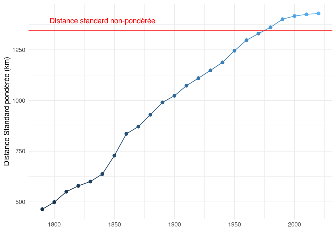
# Graphique des distances standards
pond_sd_line <- ggplot(center_pondered, aes(x = year, y = cw_sd_km, color = year)) +
geom_line() +
geom_point(size = 2) +
geom_hline(
yintercept = center_unpondered$c_sd_km, color = "red"
) +
annotate(
"text",
x = min(as.numeric(center_pondered$year)) + 50,
y = center_unpondered$c_sd_km + 50,
label = "Distance standard non-pondérée",
color = "red"
) +
labs(x = "", y = "Distance Standard pondérée (km)") +
theme_minimal() +
theme(legend.position = "none")
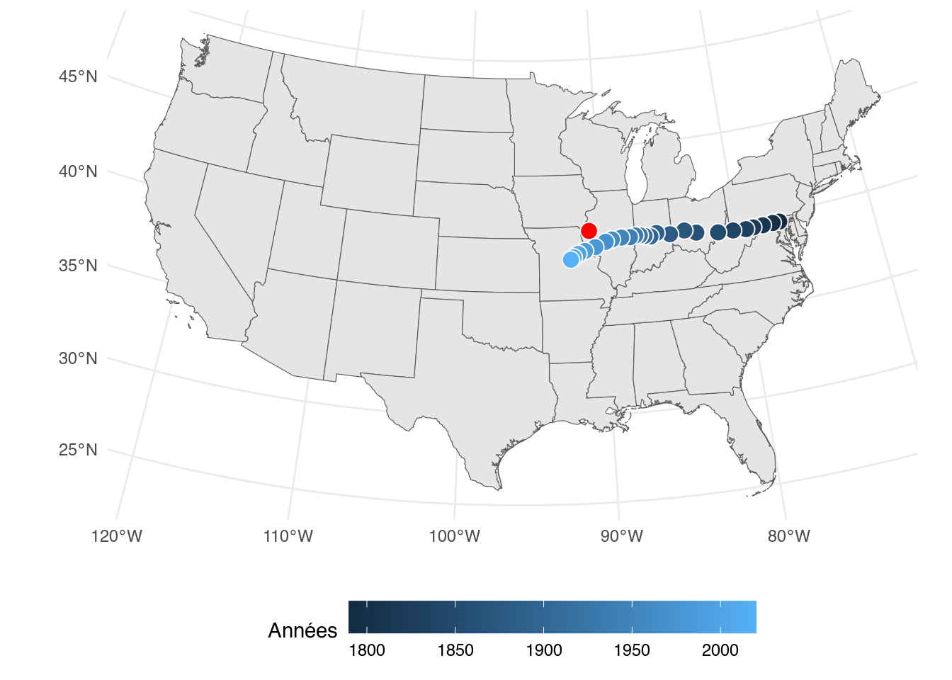
# Cartographie des centres pondérés
pond_map_disc <- ggplot() +
geom_sf(data = states) +
geom_point(
data = center_pondered,
aes(x = cw_x, y = cw_y, fill = year),
color = "white", shape = 21, size = 4
) +
geom_point(
data = center_unpondered,
aes( x = c_x, y = c_y),
color = "white", shape = 21, fill = "red", size = 4
) +
guides(fill = guide_colorbar(barwidth = 15)) +
labs(x = "", y = "", fill = "Années") +
theme_minimal() +
theme(legend.position = "bottom")
# Jointure du graphique et de la carte
wrap_plots(
list(pond_map_disc, pond_sd_line),
ncol = 1
) +
plot_annotation(
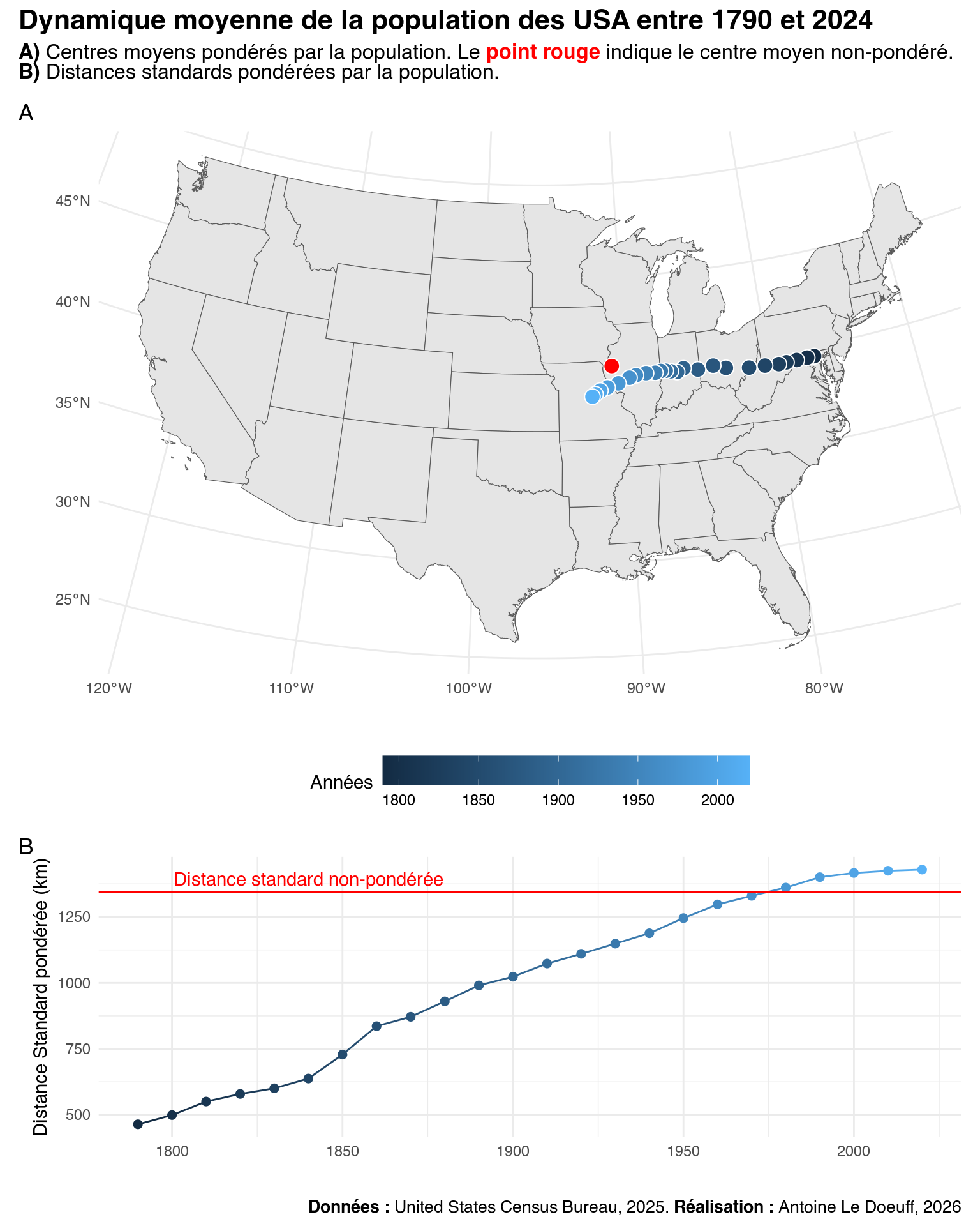
title = "Dynamique moyenne de la population des USA entre 1790 et 2024",
subtitle = "**A)** Centres moyens pondérés par la population. Le <span style='color:red;'>**point rouge**</span> indique le centre moyen non-pondéré.<br>**B)** Distances standards pondérées par la population.",
caption = "**Données :** United States Census Bureau, 2025. **Réalisation :** Antoine Le Doeuff, 2026",
tag_levels = 'A',
theme = theme(
plot.title = element_text(size = 16, face = "bold"),
plot.subtitle = ggtext::element_markdown(size = 12),
plot.caption = ggtext::element_markdown(size = 10),
)
) +
plot_layout(
heights = c(4, 2)
)
# //////////////////////////////////////////////////////////////////////////////
# Animation --------------------------------------------------------------------
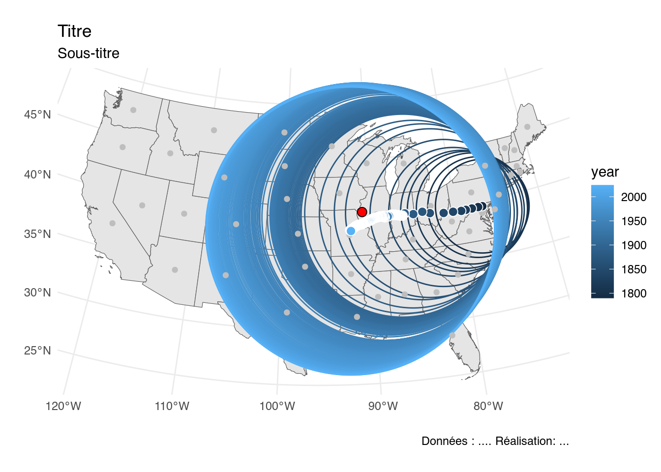
p <- ggplot() +
geom_sf(data = states) +
geom_point(
data = center_pondered,
aes(x = cw_x, y = cw_y),
color = "red", size = 4
) +
geom_text(
data = center_pondered,
aes(x = cw_x, y = cw_y, label = year),
color = "red", vjust = -1, size = 4
) +
ggforce::geom_circle(
data = center_pondered,
aes(x0 = cw_x, y0 = cw_y, r = cw_sd),
fill = "transparent", color = "black", inherit.aes = FALSE,
linewidth = 1
) +
labs(
title = "Centre moyen pondéré de la population des États-Unis",
subtitle = "Le cercle représente la distance standard pondérée. Année : {closest_state}",
x = "", y = "",
caption = "Données : United States Census Bureau, 2025. Réalisation : Antoine Le Doeuff, 2026"
) +
theme_minimal() +
theme(
plot.title = element_text(size = 18, face = "bold"),
plot.subtitle = element_text(size = 14, face = "italic"),
) +
transition_states(year) +
shadow_mark(
past = TRUE,
alpha = 0.3,
colour = "red",
exclude_layer = c(3, 4)
)
# Rendre l'animation
anim <- animate(
p,
duration = 10,
fps = 20,
width = 800,
height = 500,
renderer = gifski_renderer("figures/weighted_center.gif")
)