Stop identification with ST-DBSCAN • stdbscan

library(stdbscan)
library(readr)
library(lubridate)
library(ggplot2)
library(plotly)

Presentation

This vignette briefly demonstrates how to perform stop identification in a GPS track using ST-DBSCAN, which is a classic application of this algorithm.

Dataset

The GeoLife GPS Trajectories dataset is used for this demonstration. The GPS trajectories are located in Beijing. We previously converted the pings to a metric coordinate reference system (EPSG:4586) and selected only the relevant variables.

head(geolife_traj)
#>         date     time        x       y
#> 1 2008-10-23 02:53:04 441782.8 4428131
#> 2 2008-10-23 02:53:10 441785.6 4428129
#> 3 2008-10-23 02:53:15 441782.8 4428129
#> 4 2008-10-23 02:53:20 441780.1 4428130
#> 5 2008-10-23 02:53:25 441769.6 4428126
#> 6 2008-10-23 02:53:30 441749.3 4428121

ggplot() +
  geom_path(data = geolife_traj, aes(x, y)) +
  labs(x = "", y = "",
    title = "GPS track analyzed in this vignette",
    caption = "Data: GeoLife GPS Trajectories (Microsoft, 2012). Author: Antoine Le Doeuff, 2026",
  ) +
  coord_equal() +
  theme_minimal() +
  theme(plot.title = element_text(size = 16, face = "bold"))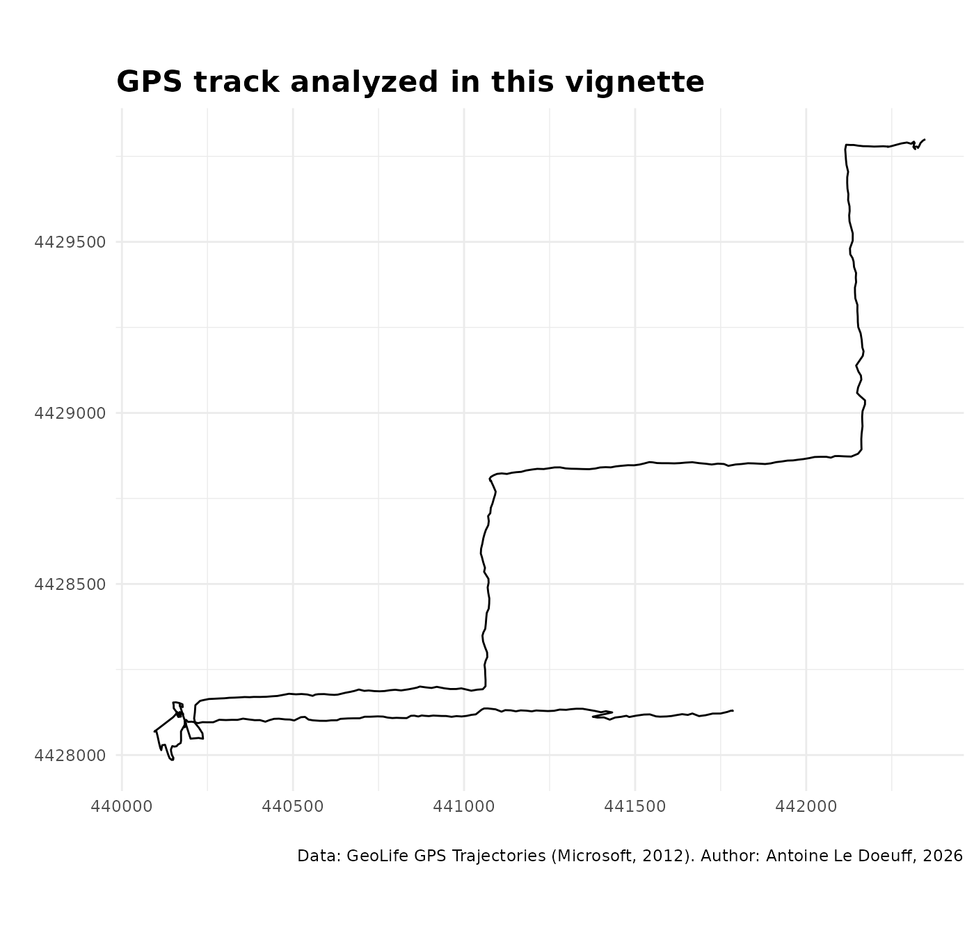

Preprocessing

For stdbscan to work, the time variable must be numeric. We therefore convert it to seconds since the beginning of the track.

geolife_traj$date_time <- as_datetime(
  paste(geolife_traj$date, geolife_traj$time), tz = "GMT"
)
geolife_traj$t <- as.numeric(
  geolife_traj$date_time - min(geolife_traj$date_time)
)

Run ST-DBSCAN

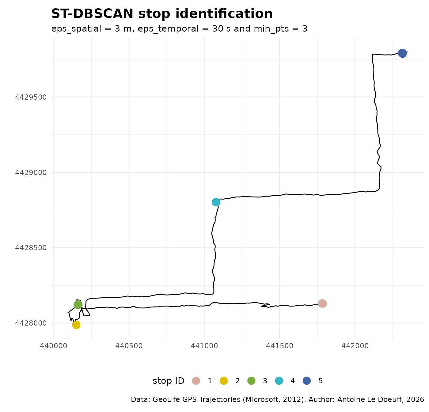
We can then run ST-DBSCAN using st_dbscan(). We set a spatial neighborhood of 3 meters, a temporal neighborhood of 30 seconds, and require a minimum of 3 pings to form a cluster. Note that these parameters are used only for demonstration purposes; in practice, a grid search (or similar tuning strategy) should be used to determine optimal values.

clusters <- st_dbscan(
  x = geolife_traj$x,
  y = geolife_traj$y,
  t = geolife_traj$t,
  eps_spatial = 3, # meters
  eps_temporal = 30, # seconds
  min_pts = 3
)
geolife_traj$clust <- as.factor(clusters)

Check result

We can check the number of pings in each cluster using table().

table(geolife_traj$clust)
#> 
#>  -1   1   2   3   4   5 
#> 420   4   5  12  12  15

Clusters can be plotted directly using ggplot2 :

# Extract stops and movements
geolife_traj_mvt <- geolife_traj[geolife_traj$clust == "-1", ]
geolife_traj_stop <- geolife_traj[geolife_traj$clust != "-1", ]

# Plot
ggplot() +
  geom_path(data = geolife_traj_mvt, aes(x, y)) +
  geom_point(data = geolife_traj_stop, aes(x, y, color = clust), size = 4) +
  labs(x = "", y = "", color = "stop ID",
    title = "ST-DBSCAN stop identification",
    subtitle = "eps_spatial = 3 m, eps_temporal = 30 s and min_pts = 3",
    caption = "Data: GeoLife GPS Trajectories (Microsoft, 2012). Author: Antoine Le Doeuff, 2026",
  ) +
  scale_color_manual(values = MetBrewer::met.brewer("Isfahan2", 5)) +
  coord_equal() +
  theme_minimal() +
  theme(
    legend.position = "bottom",
    plot.title = element_text(size = 16, face = "bold"),
  )

Clusters can be visualized in 3D using plotly :

# Zoom on stop 4
geolife_traj_f <- geolife_traj[
  geolife_traj$x > 441060 & geolife_traj$x < 441100,
]
geolife_traj_f <- geolife_traj_f[
  geolife_traj_f$y > 4428780 & geolife_traj_f$y < 4428820,
]

# Extract stop
geolife_traj_f_stop <- geolife_traj_f[geolife_traj_f$clust != "-1", ]

# Plotly figure
fig <- plot_ly(
  data = geolife_traj_f,
  x = ~x,
  y = ~y,
  z = ~t,
  type = "scatter3d", mode = "lines+markers",
  line = list(wigeolife_trajh = 4, color = "grey"),
  marker = list(size = 3, color = "grey")
)
fig |>
  add_markers(
    x = ~geolife_traj_f_stop$x,
    y = ~geolife_traj_f_stop$y,
    z = ~geolife_traj_f_stop$t,
    marker = list(size = 4, color = 'red'),
    name = 'Stop'
  ) |>
  layout(
    scene = list(
      xaxis = list(title = "x"),
      yaxis = list(title = "y"),
      zaxis = list(title = "t")
  )
)